K-mer counting tool

This post contains a short analysis of 4 FASTA files each containing a single nucleotide sequence. The goal of the analysis is to determine if the sequences have a balanced number of k-mer (4-mer) counts. The post also includes instructions on how to use the kmer_counting_tool.R script as a command line tool that lets the user select an input FASTA file and a k-mer length, and returns a file counts for each kmer sequence.
Import the FASTA files with the Biostrings package
The nucleotide sequences are imported into R as DNAStringSet objects but I will convert them into a data frame and then slice the sequences into k-mers.
#101010 black
#FDF7F7 white
library("Biostrings")
library(tidyverse)
library(gt)
library(patchwork)
theme_set(theme_light())
exp1 <- readDNAStringSet('takehome/challenge1/experiment1.fasta')
exp1## DNAStringSet object of length 1:
## width seq names
## [1] 10000 GTATTTACAGCAAAATTATATAT...ACTGCCATTTTGTCTTTTATGAGexp2 <- readDNAStringSet('takehome/challenge1/experiment2.fasta')
exp3 <- readDNAStringSet('takehome/challenge1/experiment3.fasta')
exp4 <- readDNAStringSet('takehome/challenge1/experiment4.fasta')
#exp5 = readDNAStringSet("nonstandard_nucs.fasta")
fasta_files = list(exp1, exp2, exp3, exp4)
#Function:
#convert_to_tibble()
convert_to_tibble <- function(s) {
seq_name <- names(s)
sequence <- paste(s)
df <- tibble(seq_name, sequence)
}
fasta_df <- map_df(fasta_files, convert_to_tibble)
fasta_df$seq_name = c('exp1', 'exp2', 'exp3', 'exp4')
# https://github.com/tidyverse/stringr/issues/292
str_dice <- function(s, length) { # does not return list
L <- str_length(s)
str_sub(s, start=seq(1L,L-length+1,length), end=seq(length,L,length))
}
#Function:
#kmer_len()
kmer_len <- function(tbl) {
tbl %>%
str_dice(length = 4) %>%
tibble() %>%
rename(kmer = ".") %>%
count(kmer, sort = T, name = 'kmer_count') %>%
mutate(kmer = fct_reorder(kmer, kmer_count)) %>%
mutate(standard_nucs = str_detect(kmer, "[non_stand_nucs]", negate = T))
}Table of K-mer counts by Experiment
This table is similar to the tab separated output file that is produced from the kmer_counting_tool.R where Exp1 = sequence 1 counts, etc.
seq1 <- fasta_df$sequence[1] %>%
   kmer_len() %>%
   mutate(experiment = 'Exp1_counts')

 seq2 <- fasta_df$sequence[2] %>%
  kmer_len() %>%
   mutate(experiment = 'Exp2_counts')

 seq3 <- fasta_df$sequence[3] %>%
  kmer_len() %>%
   mutate(experiment = 'Exp3_counts')

 seq4 <- fasta_df$sequence[4] %>%
  kmer_len() %>%
   mutate(experiment = 'Exp4_counts')

sequences <- bind_rows(seq1, seq2, seq3, seq4)

sequences %>%
  pivot_wider(names_from = experiment, values_from = kmer_count) %>%
  gt() %>%
  tab_header(title = md("**Kmer counts by experiment**"))  %>%
  tab_options(container.height = 400,
              container.overflow.y = TRUE,
              heading.background.color = "#EFFBFC",
              table.width = "75%",
              column_labels.background.color = "black",
              table.font.color = "black") %>%
  tab_style(style = list(cell_fill(color = "Grey")),
locations = cells_body())| Kmer counts by experiment | |||||
|---|---|---|---|---|---|
| kmer | standard_nucs | Exp1_counts | Exp2_counts | Exp3_counts | Exp4_counts |
| ATAA | TRUE | 77 | 45 | 22 | 10 |
| TAAT | TRUE | 73 | 37 | 19 | 8 |
| ATAT | TRUE | 66 | 38 | 24 | 9 |
| TATT | TRUE | 66 | 28 | 27 | 11 |
| AAAT | TRUE | 65 | 30 | 22 | 14 |
| AATT | TRUE | 65 | 36 | 15 | 11 |
| TTTT | TRUE | 63 | 29 | 28 | 9 |
| TAAA | TRUE | 60 | 30 | 24 | 9 |
| ATTT | TRUE | 58 | 33 | 24 | 7 |
| TTAT | TRUE | 57 | 48 | 23 | 8 |
| AATA | TRUE | 55 | 39 | 15 | 7 |
| AAAA | TRUE | 53 | 45 | 25 | 6 |
| ATTA | TRUE | 53 | 32 | 18 | 7 |
| TTTA | TRUE | 53 | 36 | 23 | 10 |
| TATA | TRUE | 50 | 34 | 17 | 5 |
| TTAA | TRUE | 49 | 37 | 21 | 9 |
| GATT | TRUE | 26 | 14 | 12 | 8 |
| GTTT | TRUE | 25 | 21 | 19 | 15 |
| TACT | TRUE | 24 | 14 | 16 | 12 |
| ACTA | TRUE | 22 | 19 | 15 | 7 |
| ATAC | TRUE | 22 | 19 | 11 | 9 |
| ATGA | TRUE | 22 | 17 | 13 | 6 |
| TACA | TRUE | 21 | 19 | 10 | 14 |
| TGTT | TRUE | 21 | 13 | 12 | 13 |
| ACTT | TRUE | 20 | 14 | 11 | 11 |
| CTAA | TRUE | 20 | 16 | 16 | 10 |
| AAGT | TRUE | 19 | 10 | 14 | 16 |
| CATA | TRUE | 19 | 15 | 18 | 10 |
| GAAA | TRUE | 19 | 14 | 10 | 11 |
| GTAT | TRUE | 19 | 13 | 16 | 10 |
| TAAC | TRUE | 19 | 14 | 15 | 12 |
| TCAA | TRUE | 19 | 16 | 14 | 12 |
| ACAT | TRUE | 18 | 21 | 19 | 8 |
| AGTT | TRUE | 18 | 22 | 19 | 9 |
| CTAT | TRUE | 18 | 15 | 14 | 5 |
| TTGT | TRUE | 18 | 15 | 12 | 8 |
| AACA | TRUE | 17 | 12 | 15 | 9 |
| AGAT | TRUE | 17 | 18 | 15 | 8 |
| CATT | TRUE | 17 | 22 | 13 | 6 |
| CTTT | TRUE | 17 | 12 | 8 | 8 |
| TAAG | TRUE | 17 | 22 | 18 | 7 |
| TAGA | TRUE | 17 | 15 | 15 | 7 |
| TTTG | TRUE | 17 | 20 | 14 | 10 |
| AAAC | TRUE | 16 | 17 | 10 | 13 |
| AAAG | TRUE | 16 | 18 | 12 | 9 |
| AACT | TRUE | 16 | 16 | 21 | 11 |
| ACAA | TRUE | 16 | 16 | 12 | 5 |
| ATCT | TRUE | 16 | 12 | 16 | 10 |
| GTAA | TRUE | 16 | 11 | 11 | 13 |
| GTTA | TRUE | 16 | 14 | 11 | 11 |
| TGAA | TRUE | 16 | 20 | 12 | 14 |
| TGTA | TRUE | 16 | 17 | 13 | 12 |
| TTAG | TRUE | 16 | 16 | 9 | 6 |
| TTCT | TRUE | 16 | 21 | 9 | 13 |
| AAGA | TRUE | 15 | 22 | 16 | 9 |
| CAAA | TRUE | 15 | 23 | 11 | 14 |
| TCTA | TRUE | 15 | 12 | 14 | 12 |
| TGAT | TRUE | 15 | 12 | 13 | 9 |
| TTAC | TRUE | 15 | 13 | 11 | 7 |
| TTGA | TRUE | 15 | 14 | 10 | 10 |
| ATTG | TRUE | 14 | 14 | 16 | 9 |
| CAAT | TRUE | 14 | 16 | 16 | 10 |
| CTTA | TRUE | 14 | 25 | 13 | 7 |
| GAAT | TRUE | 14 | 19 | 9 | 9 |
| GATA | TRUE | 14 | 17 | 18 | 10 |
| TATC | TRUE | 14 | 12 | 18 | 7 |
| TCTT | TRUE | 14 | 15 | 13 | 13 |
| TTTC | TRUE | 14 | 27 | 12 | 6 |
| AGTA | TRUE | 13 | 15 | 10 | 12 |
| TAGT | TRUE | 13 | 12 | 15 | 7 |
| TATG | TRUE | 13 | 23 | 18 | 10 |
| AATG | TRUE | 12 | 14 | 12 | 10 |
| AGAA | TRUE | 12 | 26 | 16 | 10 |
| ATCA | TRUE | 12 | 20 | 10 | 9 |
| ATTC | TRUE | 12 | 14 | 15 | 14 |
| TCAT | TRUE | 12 | 20 | 14 | 13 |
| AATC | TRUE | 11 | 17 | 11 | 9 |
| ATAG | TRUE | 11 | 18 | 14 | 9 |
| TTCA | TRUE | 11 | 11 | 11 | 12 |
| ATGT | TRUE | 10 | 18 | 10 | 10 |
| CATC | TRUE | 9 | 13 | 8 | 11 |
| CGTA | TRUE | 9 | 6 | 10 | 13 |
| CTCT | TRUE | 9 | 8 | 9 | 7 |
| GTCA | TRUE | 9 | 3 | 6 | 6 |
| GTCT | TRUE | 9 | 4 | 5 | 10 |
| CAAC | TRUE | 8 | 5 | 11 | 9 |
| CCAA | TRUE | 8 | 5 | 8 | 15 |
| CGAA | TRUE | 8 | 10 | 7 | 11 |
| TCCT | TRUE | 8 | 9 | 16 | 9 |
| TGAC | TRUE | 8 | 9 | 14 | 7 |
| AGTG | TRUE | 7 | 14 | 4 | 10 |
| ATCC | TRUE | 7 | NA | 12 | 14 |
| GAAG | TRUE | 7 | 7 | 6 | 7 |
| GACA | TRUE | 7 | 4 | 12 | 9 |
| GAGT | TRUE | 7 | 4 | 10 | 9 |
| GCAA | TRUE | 7 | 8 | 7 | 13 |
| GTGA | TRUE | 7 | 10 | 10 | 12 |
| TCAG | TRUE | 7 | 7 | 9 | 6 |
| AAGC | TRUE | 6 | 6 | 6 | 7 |
| AAGG | TRUE | 6 | 1 | 4 | 13 |
| ACAC | TRUE | 6 | 12 | 7 | 8 |
| ACAG | TRUE | 6 | 9 | 6 | 6 |
| ACCA | TRUE | 6 | 2 | 9 | 9 |
| AGGT | TRUE | 6 | 7 | 9 | 11 |
| CAAG | TRUE | 6 | 7 | 10 | 7 |
| GAAC | TRUE | 6 | 11 | 9 | 7 |
| GCAT | TRUE | 6 | 6 | 13 | 15 |
| TACC | TRUE | 6 | 4 | 8 | 14 |
| ACGT | TRUE | 5 | 5 | 10 | 14 |
| ACTG | TRUE | 5 | 7 | 11 | 7 |
| AGAC | TRUE | 5 | 5 | 11 | 17 |
| AGCT | TRUE | 5 | 11 | 9 | 8 |
| ATGG | TRUE | 5 | 3 | 13 | 17 |
| CACT | TRUE | 5 | 7 | 7 | 13 |
| CAGT | TRUE | 5 | 4 | 6 | 12 |
| CATG | TRUE | 5 | 8 | 12 | 5 |
| CTGT | TRUE | 5 | 13 | 11 | 10 |
| GACT | TRUE | 5 | 14 | 5 | 11 |
| GATG | TRUE | 5 | 9 | 11 | 16 |
| GGTA | TRUE | 5 | 4 | 11 | 8 |
| TAGC | TRUE | 5 | 4 | 14 | 10 |
| TCAC | TRUE | 5 | 3 | 10 | 6 |
| TGCT | TRUE | 5 | 5 | 7 | 7 |
| TGTC | TRUE | 5 | 6 | 13 | 15 |
| AACG | TRUE | 4 | 10 | 9 | 9 |
| ACGA | TRUE | 4 | 8 | 6 | 6 |
| AGGA | TRUE | 4 | 12 | 11 | 9 |
| CGTT | TRUE | 4 | 6 | 10 | 12 |
| CTTC | TRUE | 4 | 5 | 12 | 12 |
| GCTT | TRUE | 4 | 3 | 10 | 8 |
| GGTT | TRUE | 4 | 8 | 10 | 10 |
| GTTC | TRUE | 4 | 12 | 12 | 12 |
| TCTG | TRUE | 4 | 5 | 5 | 13 |
| TGAG | TRUE | 4 | 8 | 5 | 10 |
| TGCA | TRUE | 4 | 8 | 6 | 5 |
| TTCG | TRUE | 4 | 6 | 9 | 10 |
| ACTC | TRUE | 3 | 8 | 5 | 15 |
| AGAG | TRUE | 3 | 4 | 5 | 5 |
| AGCA | TRUE | 3 | 11 | 7 | 10 |
| AGTC | TRUE | 3 | 6 | 14 | 8 |
| CACA | TRUE | 3 | 6 | 5 | 8 |
| CACG | TRUE | 3 | 2 | 5 | 11 |
| CCTA | TRUE | 3 | 7 | 9 | 11 |
| CCTT | TRUE | 3 | 10 | 5 | 12 |
| CGGA | TRUE | 3 | 3 | 5 | 6 |
| CTAC | TRUE | 3 | 8 | 9 | 10 |
| CTGA | TRUE | 3 | 5 | 4 | 11 |
| GACG | TRUE | 3 | 5 | 4 | 12 |
| GATC | TRUE | 3 | 9 | 14 | 8 |
| GCCA | TRUE | 3 | 4 | 8 | 10 |
| GGAT | TRUE | 3 | 8 | 7 | 13 |
| GGCA | TRUE | 3 | 5 | 7 | 6 |
| GGGT | TRUE | 3 | 1 | 7 | 9 |
| GTAC | TRUE | 3 | 8 | 9 | 8 |
| GTAG | TRUE | 3 | 5 | 9 | 7 |
| TAGG | TRUE | 3 | 4 | 6 | 7 |
| TCGA | TRUE | 3 | 7 | 4 | 12 |
| TCTC | TRUE | 3 | 7 | 12 | 13 |
| TGGT | TRUE | 3 | 7 | 11 | 9 |
| TGTG | TRUE | 3 | 6 | 8 | 13 |
| TTGG | TRUE | 3 | 6 | 10 | 9 |
| AACC | TRUE | 2 | 6 | 12 | 12 |
| ACCT | TRUE | 2 | 6 | 8 | 10 |
| ACGG | TRUE | 2 | 1 | 6 | 7 |
| ATCG | TRUE | 2 | 7 | 8 | 10 |
| ATGC | TRUE | 2 | 7 | 10 | 11 |
| CACC | TRUE | 2 | 2 | 4 | 14 |
| CAGA | TRUE | 2 | 9 | 5 | 11 |
| CCAT | TRUE | 2 | 1 | 14 | 8 |
| CGAT | TRUE | 2 | 7 | 5 | 13 |
| CGCC | TRUE | 2 | 1 | 4 | 6 |
| CTAG | TRUE | 2 | 10 | 7 | 6 |
| CTGC | TRUE | 2 | 1 | 6 | 12 |
| CTTG | TRUE | 2 | 4 | 8 | 13 |
| GCAC | TRUE | 2 | 5 | 6 | 10 |
| GCCT | TRUE | 2 | 4 | 10 | 12 |
| GCTA | TRUE | 2 | 4 | 6 | 12 |
| GGAA | TRUE | 2 | 7 | 9 | 12 |
| GGAC | TRUE | 2 | 7 | 12 | 12 |
| GTCC | TRUE | 2 | 3 | 6 | 8 |
| GTGT | TRUE | 2 | 8 | 9 | 11 |
| GTTG | TRUE | 2 | 11 | 10 | 9 |
| TACG | TRUE | 2 | 9 | 8 | 9 |
| TCCA | TRUE | 2 | 9 | 18 | 10 |
| TCCG | TRUE | 2 | 1 | 9 | 7 |
| TCGC | TRUE | 2 | 1 | 6 | 9 |
| TGCG | TRUE | 2 | 3 | 5 | 8 |
| TTCC | TRUE | 2 | 2 | 7 | 10 |
| TTGC | TRUE | 2 | 8 | 6 | 9 |
| ACCG | TRUE | 1 | 1 | 8 | 12 |
| ACGC | TRUE | 1 | 4 | 6 | 6 |
| AGCC | TRUE | 1 | 3 | 10 | 6 |
| AGGC | TRUE | 1 | NA | 5 | 7 |
| CAGC | TRUE | 1 | 4 | 4 | 6 |
| CCAC | TRUE | 1 | 2 | 3 | 12 |
| CCAG | TRUE | 1 | 1 | 10 | 11 |
| CCCC | TRUE | 1 | NA | 5 | 5 |
| CCCT | TRUE | 1 | 3 | 8 | 8 |
| CCTC | TRUE | 1 | 2 | 6 | 12 |
| CGAC | TRUE | 1 | 2 | 6 | 11 |
| CGCT | TRUE | 1 | 1 | 4 | 12 |
| CGGT | TRUE | 1 | 3 | 2 | 11 |
| CTCA | TRUE | 1 | 7 | 6 | 9 |
| CTCC | TRUE | 1 | 2 | 2 | 7 |
| CTCG | TRUE | 1 | 3 | 5 | 8 |
| GACC | TRUE | 1 | NA | 2 | 6 |
| GAGA | TRUE | 1 | 4 | 9 | 11 |
| GAGC | TRUE | 1 | 2 | 9 | 9 |
| GCGA | TRUE | 1 | NA | 6 | 12 |
| GCGT | TRUE | 1 | 3 | 4 | 7 |
| GCTC | TRUE | 1 | 1 | 5 | 13 |
| GGAG | TRUE | 1 | 1 | 3 | 9 |
| GGCC | TRUE | 1 | 1 | 5 | 7 |
| GGGC | TRUE | 1 | 2 | 6 | 7 |
| TCGG | TRUE | 1 | NA | 5 | 9 |
| TCGT | TRUE | 1 | 9 | 9 | 12 |
| TGGA | TRUE | 1 | 4 | 14 | 8 |
| TGGG | TRUE | 1 | 4 | 5 | 8 |
| AGGG | TRUE | NA | 5 | 4 | 5 |
| CCGT | TRUE | NA | 5 | 5 | 14 |
| GGTG | TRUE | NA | 5 | 7 | 10 |
| GTGC | TRUE | NA | 5 | 3 | 6 |
| AGCG | TRUE | NA | 4 | 6 | 7 |
| CCGA | TRUE | NA | 4 | 4 | 9 |
| CCTG | TRUE | NA | 4 | 6 | 13 |
| CTGG | TRUE | NA | 4 | 7 | 17 |
| GTCG | TRUE | NA | 4 | 6 | 12 |
| GTGG | TRUE | NA | 4 | 3 | 10 |
| CCCA | TRUE | NA | 3 | 2 | 9 |
| CCGG | TRUE | NA | 3 | 2 | 9 |
| CGAG | TRUE | NA | 3 | 3 | 11 |
| CGCG | TRUE | NA | 3 | 2 | 8 |
| CGTC | TRUE | NA | 3 | 7 | 8 |
| CGTG | TRUE | NA | 3 | 4 | 3 |
| GAGG | TRUE | NA | 3 | 5 | 10 |
| GCAG | TRUE | NA | 3 | 3 | 9 |
| GCTG | TRUE | NA | 3 | 6 | 13 |
| GGGA | TRUE | NA | 3 | 5 | 11 |
| GGTC | TRUE | NA | 3 | 7 | 10 |
| TCCC | TRUE | NA | 3 | 9 | 14 |
| TGGC | TRUE | NA | 3 | 4 | 9 |
| CAGG | TRUE | NA | 2 | 2 | 8 |
| CGGG | TRUE | NA | 2 | 3 | 15 |
| GGCT | TRUE | NA | 2 | 6 | 13 |
| TGCC | TRUE | NA | 2 | 8 | 6 |
| CCCG | TRUE | NA | 1 | 2 | 9 |
| CCGC | TRUE | NA | 1 | 8 | 10 |
| CGGC | TRUE | NA | 1 | 8 | 7 |
| GCCC | TRUE | NA | 1 | 5 | 10 |
| GCCG | TRUE | NA | 1 | 6 | 7 |
| GCGG | TRUE | NA | 1 | 1 | 7 |
| GGCG | TRUE | NA | 1 | 5 | 8 |
| GGGG | TRUE | NA | 1 | 7 | 14 |
| CGCA | TRUE | NA | NA | 12 | 10 |
| ACCC | TRUE | NA | NA | 6 | 13 |
| GCGC | TRUE | NA | NA | 2 | 9 |
It may be helpful to visualize the k-mer count distributions to get a better feel for the similarities and differences between the sequences.
Bar plots of count distributions for each experiment
#Function:
#create bar plots with bar_plot()
bar_plot <- function(tbl) {
  tbl %>%
    ggplot(aes(kmer_count, kmer, fill = kmer_count)) +
    geom_col() +
    scale_fill_viridis_c() +
    theme(legend.position = 'none') +
    theme(axis.title.y = element_blank(),
          axis.text.y = element_blank(),
          axis.ticks.y = element_blank()) +
    labs(x = "K-mer counts")
}

p1 <- fasta_df$sequence[1] %>%
  kmer_len() %>%
  bar_plot() +
  labs(title = 'Exp1 kmer counts')


p2 <- fasta_df$sequence[2] %>%
  kmer_len() %>%
  bar_plot() +
  labs(title = 'Exp2 kmer counts')

p3 <- fasta_df$sequence[3] %>%
  kmer_len() %>%
  bar_plot() +
  labs(title = 'Exp3 kmer counts')

p4 <- fasta_df$sequence[4] %>%
  kmer_len() %>%
  bar_plot() +
  labs(title = 'Exp4 kmer counts')

(p1 + p2) / (p3 + p4)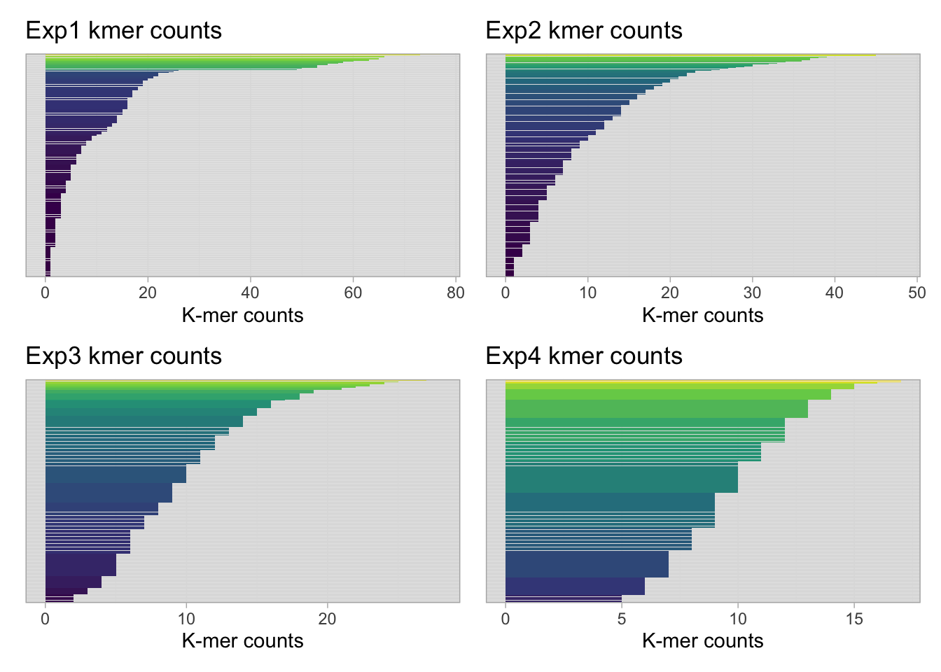
Notably, the count distributions are progressively less varied.
Summary table
The max count and sd count variation are worth exploring further.
#create a summary table with the median, min and max
sequences %>%
  group_by(experiment) %>%
  drop_na() %>%
  summarize(`median count` = median(kmer_count),
            `mean count` = round(mean(kmer_count)),
            `sd count` = round(sd(kmer_count)),
            `max count` = max(kmer_count)) %>%
  gt() %>%
  tab_header(title = md("**K-mer counts summary table**"),)  %>%
  tab_options(
              heading.background.color = "#EFFBFC",
              table.width = "75%",
              column_labels.background.color = "black",
              table.font.color = "black") %>%
  tab_style(style = list(cell_fill(color = "Grey")),
locations = cells_body())| K-mer counts summary table | ||||
|---|---|---|---|---|
| experiment | median count | mean count | sd count | max count |
| Exp1_counts | 5 | 11 | 15 | 77 |
| Exp2_counts | 7 | 10 | 9 | 48 |
| Exp3_counts | 9 | 10 | 5 | 28 |
| Exp4_counts | 10 | 10 | 3 | 17 |
Density plots
We can get a better feeling for the count distributions with density plots.
sequences %>%
  group_by(experiment) %>%
  ggplot(aes(kmer_count, fill = experiment)) +
  geom_density() +
  facet_wrap(~experiment) +
  scale_fill_viridis_d() +
  theme(legend.position = 'none') +
  labs(title = "Density distributions of k-mers (4-mers) by count",
       x = "Kmer count",
       y = "Density")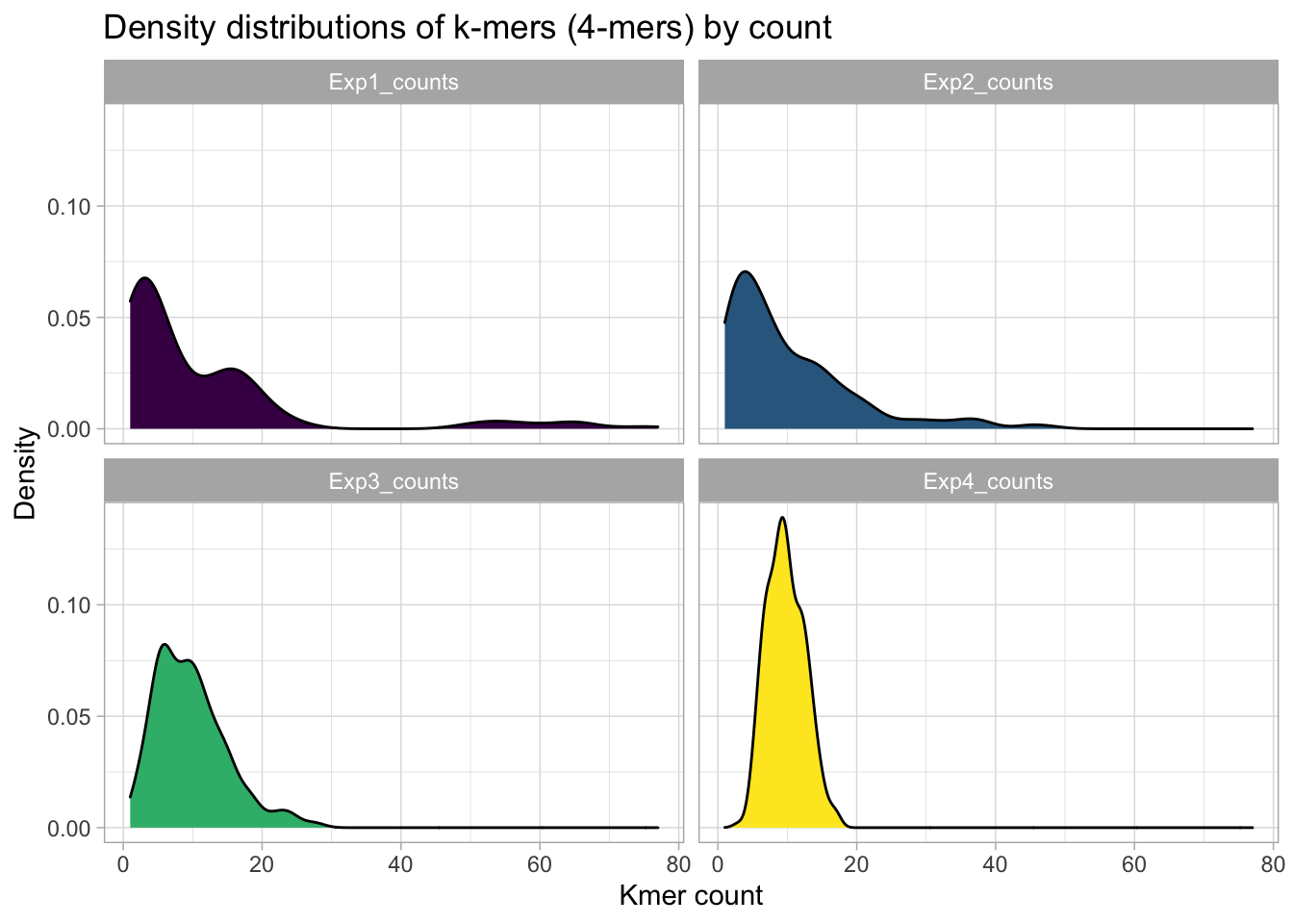
Binning the kmer counts for a more general pattern
In the next two plots, the k-mer counts are grouped into 8 categories (10-80 k-mer counts by 10 and an other category). For all experiments, most of the 256 possible k-mers appear less than 10 times. So as not to dwarf the k-mer counts that appear more than ten times, the ‘10 and under’ category is shown separately.
sequences %>%
  mutate(kmer_count = as.numeric(kmer_count),
         counts_bins40_200 = case_when(
           kmer_count <= 10 ~ as.character('10 and under'),
           between(kmer_count, 11, 20) ~ as.character('11-20'),
           between(kmer_count, 21, 30) ~ as.character('21-30'),
           between(kmer_count, 31, 40) ~ as.character('31-40'),
           between(kmer_count, 51, 60) ~ as.character('41-50'),
           between(kmer_count, 61, 70) ~ as.character('41-50'),
           kmer_count >= 71 ~ as.character('71 and greater'),
           TRUE ~ 'other'
         )) %>%
  filter(counts_bins40_200 == "10 and under", counts_bins40_200 != '11-20') %>%
  group_by(counts_bins40_200) %>%
  ggplot(aes(counts_bins40_200, fill = experiment)) +
  stat_count() +
  scale_fill_viridis_d() +
  labs(title = "Count of binned k-mers",
       subtitle = "The distribution of k-mer counts between 0-10",
       x = "K-mer count",
       y = "Density")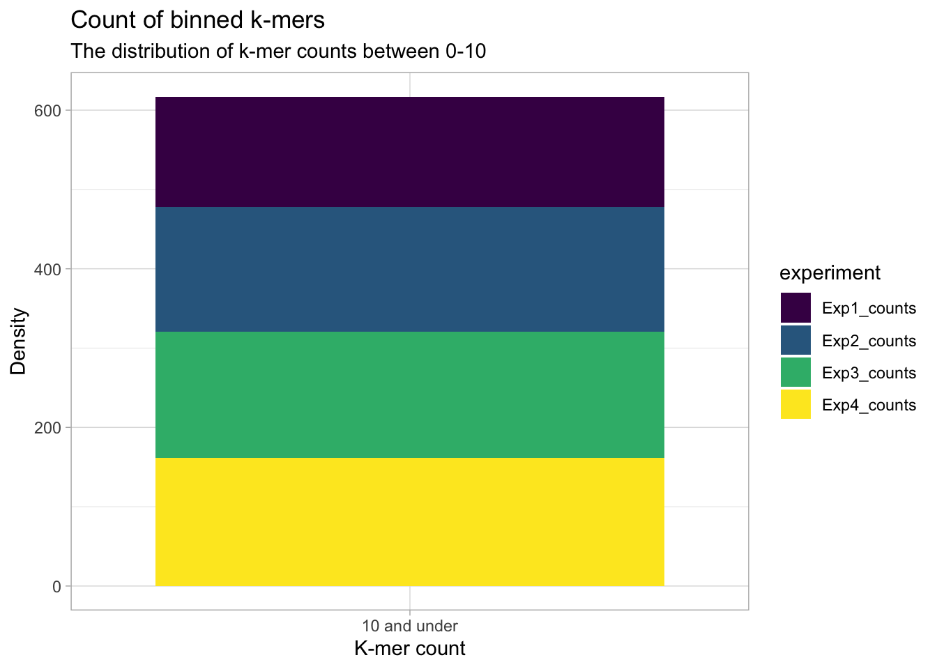
sequences %>%
  mutate(kmer_count = as.numeric(kmer_count),
         counts_bins40_200 = case_when(
           kmer_count <= 20 ~ as.character('10 and under'),
           between(kmer_count, 11, 20) ~ as.character('11-20'),
           between(kmer_count, 21, 30) ~ as.character('21-30'),
           between(kmer_count, 31, 40) ~ as.character('31-40'),
           between(kmer_count, 51, 60) ~ as.character('41-50'),
           between(kmer_count, 61, 70) ~ as.character('41-50'),
           kmer_count >= 71 ~ as.character('71 and greater'),
           TRUE ~ 'other'
         )) %>%
  filter(counts_bins40_200 != "10 and under", counts_bins40_200 != 'other') %>%
  group_by(counts_bins40_200) %>%
  ggplot(aes(counts_bins40_200, fill = experiment)) +
  stat_count() +
  scale_fill_viridis_d() +
  labs(title = "Count of binned k-mers",
       subtitle = "The distribution of kmer counts between 10-80",
       x = "K-mer count",
       y = "Density")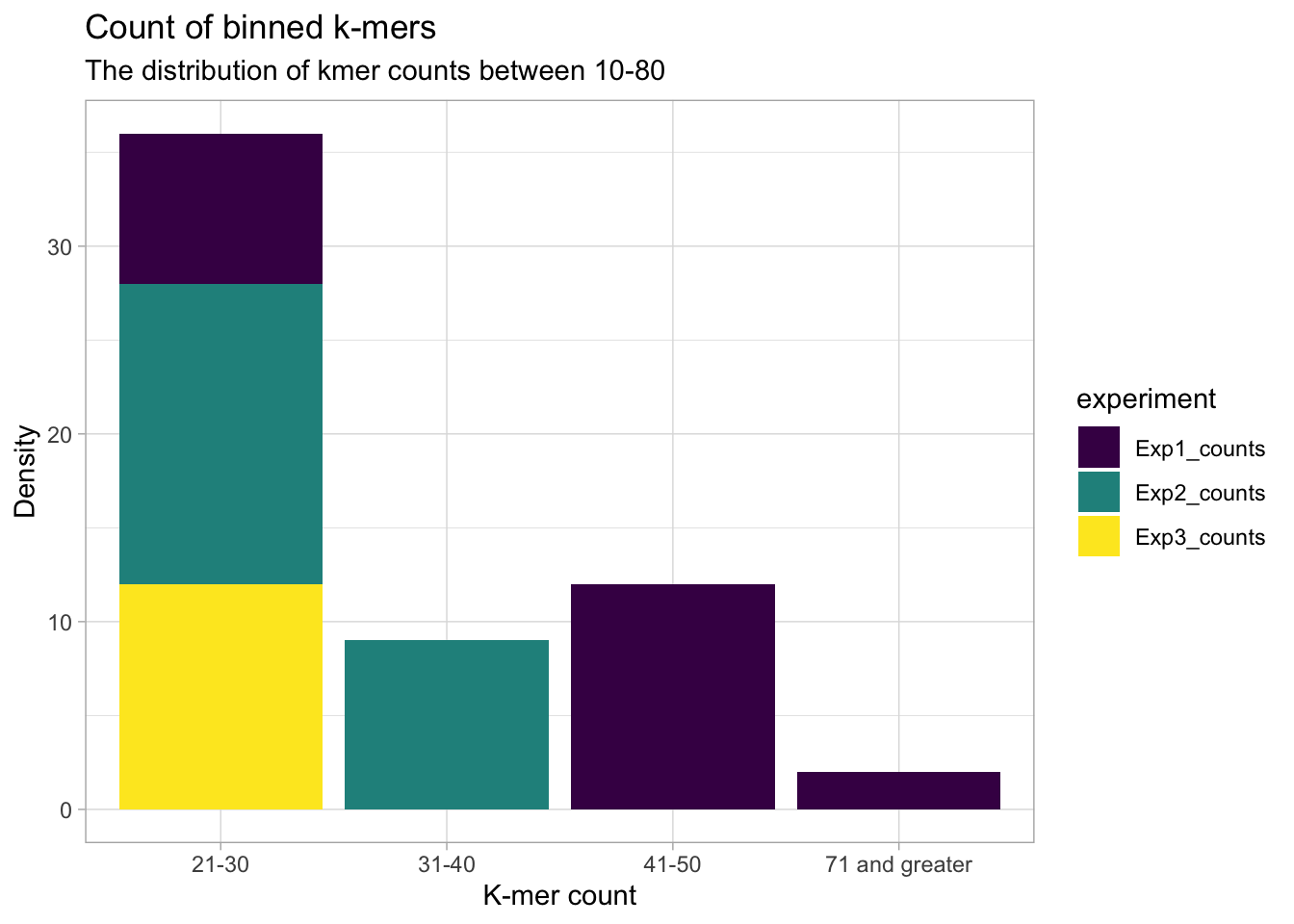
We see that experiment 2 dominates k-mer counts in the 30-40 range and experiment 1 dominates in the greater than 40 range.
Instructions: k-mer counting script for the command line
To help you check for imbalanced k-mer distributions in future experiments, I designed a k-mer counting analysis script that works from the command line. The k-mer counter let’s you input a FASTA file and k-mer length, and returns a tab separated file of k-mer counts ordered by frequency. The program also returns messages about the analysis including:
- Input sequence length
- K-mer length
- Which nonstandard nucleotides the program can identify
- Whether the k-mer length is acceptable for the sequence range
- The top 10 k-mers by count
- Whether the given sequence contains standard or nonstandard nucleotides. The nonstandard nucleotide warning can be tested with the following file: takehome/challenge1/nonstandard_nucs.fasta
To use the k-mer counting tool:
1. Download the directory I sent you and open it in the command line
2. Change the permissions for kmer_counter_tool.R script to make it executable on your machine (chmod +x kmer_counter_tool.R)
3. Then run the following incantation in your command line (with custom input and output file names):
Rscript kmer_counter_tool.R ‘input_file’ kmer-length –output_file ‘output_file’
e.g., 
4. See the image below for the expected output in the command line (Note: I am working on a mac).
When running the script, a new output file (tab separated format) with k-mers ordered by frequency is generated.

Gabriel Mednick, PhD
Data scientist, biochemist, computational biologist, educator, life enthusiast